Roman I-Sim Tutorials

This article provides examples of the basic functionalities of Roman I-Sim . Additional information is available from the tool's online documentation.
The purpose of these examples is to show how to: (1) generate catalogs of real or simulated sources; (2) generate simulated Level 1 (L1) or Level 2 (L2) Roman WFI ASDF files with Roman I-Sim ; and (3) display the output image. For more examples covering other aspects of the simulation tool, including the Roman I-Sim creation of astronomical scenes (called Level 3, L3, by the program, but not to be confused with the real Level 3 data products created using romancal ), please consult the readthedocs documentation.
Note
- L1 WFI data files contain a single uncalibrated ramp exposure in units of Digital Numbers (DN). L1 files are three-dimensional data cubes, one dimension for time and two dimensions for image coordinates, that are shaped as arrays with (N resultants, 4096 image rows, 4096 image columns).
- L2 WFI data contain calibrated rate images in instrumental units of DN per second (DN/s). They are two-dimensional arrays shaped as (4088 image rows, 4088 image columns).
Additional details about the Roman data levels can be found on the WFI Data Levels and Products RDox article.
Example 1: Creating a Catalog of Gaia Sources
The Roman I-Sim package offers two options for generating source catalogs:
- Retrieve the source catalog from Gaia; or
- Parametrically generate a catalog of stars and/or galaxies.
First, let's explore how to create a source catalog compatible with Roman I-Sim using Gaia. We will use a combination of astroquery and Roman I-Sim to query the Gaia catalog and then write the file in a format compatible with Roman I-Sim .
In our example below, we will query the Gaia DR3 catalog for sources centered at (R.A., Dec.) = (80.0, 30.0) degrees and within a radius of 1 degree.
Note
The Gaia query may take several minutes to complete depending on the search radius specified.
import argparse
from astroquery.gaia import Gaia
from astropy.coordinates import SkyCoord
from astropy.time import Time
from astropy.table import vstack
import galsim
import numpy as np
from romanisim import gaia, bandpass, catalog, log, wcs, persistence, parameters, ris_make_utils as ris


ra = 80.0     # Right ascension in degrees
dec = 30.0    # Declination in degrees
radius = 1.0  # Search radius in degrees

query = f'SELECT * FROM gaiadr3.gaia_source WHERE distance({ra}, {dec}, ra, dec) < {radius}'
job = Gaia.launch_job_async(query)

result = job.get_results()
Once we have the result from the Gaia query, we can transform it into a format compatible with Roman I-Sim . We can also optionally write it to an Enhanced Character-Separated Value (ECSV) file compatible with Roman I-Sim :
obs_time = '2026-10-31T00:00:00'
gaia_catalog = gaia.gaia2romanisimcat(result, Time(obs_time), fluxfields=set(bandpass.galsim2roman_bandpass.values()))

# Clean out bad sources from Gaia catalog:
bandpass = [f for f in gaia_catalog.dtype.names if f[0] == 'F']
bad = np.zeros(len(gaia_catalog), dtype='bool')
for b in bandpass:
     bad = ~np.isfinite(gaia_catalog[b])
     if hasattr(gaia_catalog[b], 'mask'):
          bad |= gaia_catalog[b].mask
     gaia_catalog = gaia_catalog[~bad]

gaia_catalog = gaia_catalog[np.isfinite(gaia_catalog['ra'])]

gaia_catalog.write('gaia_catalog.ecsv', overwrite=True)
The generation of a Gaia source catalog can also be run using a command-line executable, as shown below where the arguments are explicitly spelled out. More information is available in the readthedocs documentation.
romanisim-make-catalog 80.0 30.0 1.0 --time 2026-10-31T00:00:00 --output test.ecsv
For more help, use the following command line:
romanisim-make-catalog --help
Example 2: Creating a Catalog of Simulated Sources
Alternatively, we can generate a completely synthetic catalog of stars and galaxies using tools in Roman I-Sim (see parameters in the cell below).
# Galaxy catalog parameters

ra = 80.0                   # Right ascension of the catalog center in degrees
dec = 30.0                  # Declination of the catalog center in degrees
radius = 0.4                # Radius of the catalog in degrees
n_gal = 10_000              # Number of galaxies
faint_mag = 22              # Faint magnitude limit of simulated sources
hlight_radius = 0.3         # Half-light radius at the faint magnitude limit in units of arcseconds
optical_element = ['F106']  # List of optical elements to simulate
seed = 5346                 # Random number seed for reproducibility

# Additional star catalog parameters

n_star = 30_000  # Number of stars

galaxy_cat = catalog.make_galaxies(SkyCoord(ra, dec, unit='deg'), n_gal, radius=radius, index=0.4, faintmag=faint_mag,
                                   hlr_at_faintmag=hlight_radius, bandpasses=optical_element, rng=None, seed=seed)

star_cat = catalog.make_stars(SkyCoord(ra, dec, unit='deg'), n_star, radius=radius, index=5/3., faintmag=faint_mag,
                              truncation_radius=None, bandpasses=optical_element, rng=None, seed=seed)

full_catalog = vstack([galaxy_cat, star_cat])

full_catalog.write('parametric_catalog.ecsv', format='ascii.ecsv', overwrite=True)
Example 3: Generating a Simulated Image
In this example, we show how to run the actual
Roman I-Sim
simulation to generate L2 data products. The method for running the simulation for both L1 and L2 data is the same. For users interested in simulating L1 ramp cubes, the level variable below can be changed to 1, which will have an output file ending in _uncal.asdf. The rest of the information remains the same.
In our example, we are simulating only a single image, so we set the persistence to the default. Future updates may include how to simulate persistence from multiple exposures.
Note
- Roman I-Sim allows the user to either use reference files from CRDS or to use no reference files. The latter mode is not recommended because the data may lack realistic noise properties.
- Each detector is simulated separately.
- In operations, multi-accumulation (MA) tables may be truncated at specific resultants, but here we show how to simulate the full MA table. MA table 109 contains 10 resultants made up of 44 reads (a total exposure time of approximately 134 seconds) with resultants made up of 1, 2, 3, 4, and 6 resultants with the final resultant containing a single read. More information on MA tables can be found at WFI MultiAccum (MA) Tables.
First, we specify some inputs for the simulator. Note also that you will need the full catalog generated in Example 2.
# Specify WFI_CEN pointing RA and Dec.
ra = 80.0                         # Right ascension of the catalog center in degrees
dec = 30.0                        # Declination of the catalog center in degrees

obs_date = '2026-10-31T00:00:00'  # Datetime of the simulated exposure
sca = 1  # Change this number to simulate different WFI detectors 1 - 18
optical_element = 'F106'  # Optical element to simulate
ma_table_number = 1018  # Multi-accumulation (MA) table number...do not recommend to change this as it must match files in CRDS
seed = 7  # Galsim random number generator seed for reproducibility
level = 2  # WFI data level to simulate...1 or 2

cal_level = 'cal' if level == 2 else 'uncal'  # File name extension for data calibration level
filename = f'r0003201001001001004_0001_wfi{sca:02d}_{optical_element.lower()}_{cal_level}.asdf'  # Output file name on disk. Only change the first part up to _WFI to change the rootname of the file.
Then, we organize these inputs in the expected format. The last code line below is where Roman I-Sim is actually run. The resulting simulated image and corresponding metadata are saved as an ASDF file.
# Set other arguments for use in Roman I-Sim. The code expects a specific format for these, so this is a little complicated looking.
parser = argparse.ArgumentParser()
parser.set_defaults(usecrds=True, psftype='stpsf', level=level, filename=filename, drop_extra_dq=True, sca=sca, bandpass=optical_element, pretend_spectral=None)
args = parser.parse_args([])

# Set reference files to None for CRDS
for k in parameters.reference_data:
    parameters.reference_data[k] = None

# Set Galsim RNG object
rng = galsim.UniformDeviate(seed)

# Set default persistance information
persist = persistence.Persistence()

# Set metadata
metadata = ris.set_metadata(date=obs_date, bandpass=optical_element, sca=sca, ma_table_number=ma_table_number, usecrds=True)

# Update the WCS info
wcs.fill_in_parameters(metadata, SkyCoord(ra, dec, unit='deg', frame='icrs'), boresight=False, pa_aper=0.0)

# Run the simulation
ris.simulate_image_file(args, metadata, full_catalog, rng, persist)
Note
At runtime, the last command above may display a warning about "asdf-astropy" versions; you may safely ignore it
Note
Alternatively, the user may also use the following command to instead return a WfiImage object as well as a dictionary of valuable quantities, therefore avoiding saving and opening a file.
im, extras = ris.image.simulate(metadata, full_catalog, persistence=persist, seed=seed, rng=rng, psftype='stpsf', level=2)
The pixel data can then be accessed using im.data
Roman I-Sim can also be run using a command-line executable, where the arguments are explicitly spelled out. Below we provide an example, but more information is available in the readthedocs documentation.
romanisim-make-image --bandpass F106 --catalog parametric_catalog.ecsv --date 2026-10-31T00:00:00 --level 2 --ma_table_number 1018 --radec 80.0 30.0 --roll 0 --sca 1 --usecrds --psftype stpsf --rng_seed 7 ./r0003201001001001004_01101_0001_WFI01_cal_command.asdf
For more help, use the following command line:
romanisim-make-image --help
Example 4: Displaying a Simulated Image
We can now use the ASDF file created by
Roman I-Sim
and display the result using matplotlib. The code below shows how to access both the data and World Coordinate System (WCS) information from the ASDF file.
First, we open the ASDF file using Roman Datamodels:
import roman_datamodels as rdm

file = rdm.open(filename)
wfi = file.meta.instrument.detector
Next, we can display the data using matplotlib, where the result is shown below.
from astropy import visualization
from astropy import units as u

import matplotlib.pyplot as plt
import matplotlib.colors as colors
from matplotlib import colormaps as cm


cmap = cm['RdYlBu_r']

norm = visualization.ImageNormalize(file.data,
                                    interval=visualization.ZScaleInterval(contrast=0.25),
                                    stretch=visualization.AsinhStretch(a=1))

fig, ax = plt.subplots(figsize=(8, 6), subplot_kw={'projection':file.meta.wcs})

plot = ax.imshow(file.data, norm=norm, cmap=cmap, origin='lower')

ax.coords.grid(linestyle='dashed', color='grey', alpha=0.5)

lon = ax.coords[0]
lat = ax.coords[1]

lon.set_axislabel('Right Ascension')
lat.set_axislabel('Declination')

lon.set_major_formatter('d.dd')
lat.set_major_formatter('d.dd')

lon.set_ticks(spacing=2 * u.arcminute)
lat.set_ticks(spacing=2 * u.arcminute)


plt.title(f"Roman I-Sim {wfi}")

cax = plt.axes([0.825, 0.11, 0.025,0.77 ])
plt.colorbar(mappable=plot, cax=cax)

file.close()
Figure of Example Roman I-Sim Simulated Image
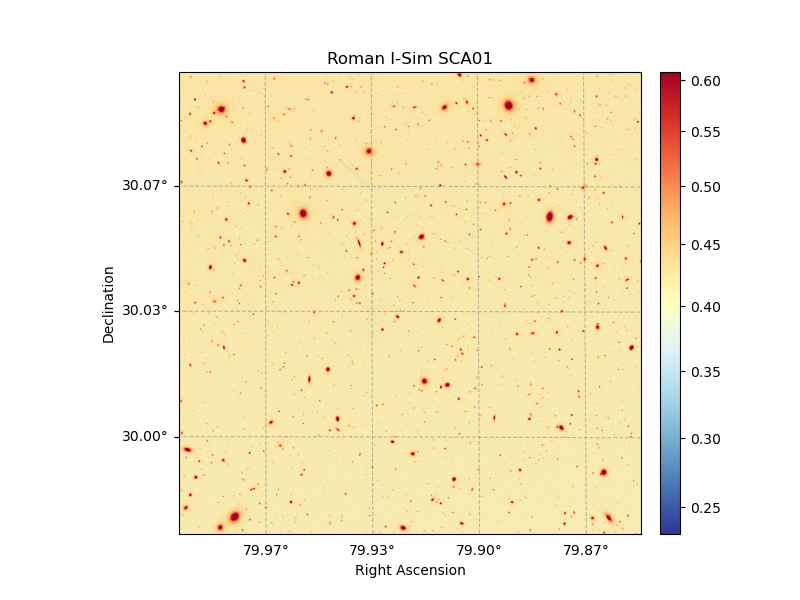
Sample image as simulated using Roman I-Sim output from the matplotlib code example.
References
- Roman I-Sim on
readthedocs: https://romanisim.readthedocs.io/en/latest/ - Gaia: https://www.esa.int/Science_Exploration/Space_Science/Gaia
For additional questions not answered in this article, please contact the Roman Help Desk.