STIPS Tutorials

The Space Telescope Imaging Product Simulator (STIPS) is a versatile tool designed to simulate exposure level astronomical scenes from the Wide Field Instrument (WFI) for Roman. This article presents a few simple examples on the functionalities of STIPS. Users can find a more extensive list of tutorials and examples in the form of python jupyter notebooks on the Roman Research Nexus (RRN). Additional information is available from the tool's online documentation and by consulting the published paper.

Important Information
STIPS is no longer under active development and is currently in maintenance mode, with updates limited to critical bug fixes. For improved fidelity with Roman observations and pipeline compatibility, we recommend transitioning to Roman I-Sim.
The Basic STIPS Usage Tutorial builds on the concepts introduced in the Overview of STIPS article and is designed to walk through the phases of using STIPS at the most introductory level: (1) creating a small astronomical scene; (2) designing an observation; and (3) generating a simulated image.
Example 1: Generating a Simple Astronomical Scene
STIPS provides functionalities to generate catalogs of stars or galaxies with user-specified input parameters. Users can also provide their own source catalogs, as described in Catalogs formatting on readthedocs.
In the example below, we show how to create an astronomical scene by passing the user-defined input catalogs to STIPS in the FITS format. The catalog contains the coordinates of the sources, the observed flux, and any necessary shape parameters. The code block below provides an example of the required input information to generate a catalog containing two point sources. The catalog is saved to a file called catalog.fits for later use.
from astropy.io import fits

cols=[]
cols.append(fits.Column(name='id'   ,array=[1,2]            , format='K' )) # Object ID
cols.append(fits.Column(name='ra'   ,array=[90.02,90.03]    , format='D' )) # RA in degrees
cols.append(fits.Column(name='dec'  ,array=[29.98,29.97]    , format='D' )) # DEC in degrees
cols.append(fits.Column(name='flux' ,array=[0.00023,0.0004] , format='D' )) # Flux in `units`
cols.append(fits.Column(name='type' ,array=['point','point'], format='8A')) # `point` or `sersic`
cols.append(fits.Column(name='n'    ,array=[0,0]            , format='D' )) # Sersic profile index
cols.append(fits.Column(name='re'   ,array=[0,0]            , format='D' )) # Half-light radius in pixels
cols.append(fits.Column(name='phi'  ,array=[0,0]            , format='D' )) # Angle of PA in degrees
cols.append(fits.Column(name='ratio',array=[0,0]            , format='D' )) # Axial Ratio
cols.append(fits.Column(name='notes',array=['','']          , format='8A')) # Notes
cols.append(fits.Column(name='units',array=['j','j']        , format='8A')) # Units, 'j' for jansky

# Create output fits table
hdut = fits.BinTableHDU.from_columns(cols)
hdut.header['TYPE']='mixed'
hdut.header['FILTER']='F129'

# Write to disk
hdut.writeto('catalog.fits',overwrite=True)
The output of this code block is a FITS table containing the generated catalog of sources.
Example 2: Observation Setup
Next, we prepare inputs for the scene we created above. We use the ObservationModule to generate an observation object. We generate an obs dictionary containing the properties of the observation (e.g. the instrument and the detector setups) and parameters describing central coordinates (R.A., Dec.), position angle (PA), and computational parameters for the simulation.
The Observation Dictionary
An example obs dictionary is specified in the code block below. In this example, we select:
- The imaging filter F129
- The WFI01 detector
- Sky background from Pandeia
- An observation ID of 42
- An exposure time of 300 seconds
Together with the following single offset setting:
- An offset ID of 1
- No centering
- No changes in R.A., Dec., and PA from the center of the observation
from stips.observation_module import ObservationModule

# Build observation parameters
obs = {'instrument'       : 'WFI',
       'filters'          : ['F129'],
       'detectors'        : 1,
       'background'       : 'pandeia',
       'observations_id'  : 42,
       'exptime'          : 300,
       'offsets'          : [{'offset_id'    : 1    ,
                              'offset_centre': False,
                              'offset_ra'    : 0.0  ,
                              'offset_dec'   : 0.0  ,
                              'offset_pa'    : 0.0  }]}
The Observation Object
An observation object combines the obs dictionary with the central coordinates (RA, Dec), orientation angle, and computational parameters for the simulation. Then, the setup can be initialized.
# Create observation object
obm = ObservationModule(obs,
                        ra    = 90,
                        dec   = 30,
                        pa    = 0,
                        seed  = 42,
                        cores = 6)
Example 3: Generating a Simulated Image
The code block below combines the inputs required for
STIPS
that were generated above and finalizes the
ObservationModule
to run a simulation. The final simulated image will be saved under the name specified by the
fits_file
variable, and the result is shown on the right.
import numpy as np
import matplotlib.pyplot as plt
from astropy.io import fits

# Initialize the local instrument
obm.nextObservation()

# Add catalog with sources
cat_name = obm.addCatalogue('catalog.fits')

# Add error to image
psf_file = obm.addError()

# Call the final method
fits_file, mosaic_file, params = obm.finalize(mosaic=False)
print("Output FITS file is {}".format(fits_file))

# memory-safe way of reading the file
with fits.open(fits_file, mode='readonly') as hdul:
	data = hdul[1].data

# Plot the simulated FITS image
fig, ax = plt.subplots(2, 1, figsize=(16, 10))

vmin = np.percentile(data, 5)
vmax = np.percentile(data, 95)

ax[0].imshow(data,
             origin="lower",
             cmap="grey",
             vmin=vmin,
             vmax=vmax)

ax[1].imshow(data,
             origin="lower",
             cmap="grey",
             vmin=vmin,
             vmax=vmax)

ax[1].set_xlim(2300, 3300)
ax[1].set_ylim(700, 1700)

ax[0].set_xlabel("X [pixels]")
ax[0].set_ylabel("Y [pixels]")

ax[1].set_xlabel("X [pixels]")
ax[1].set_ylabel("Y [pixels]")

plt.suptitle("Output Simulated FITS image")
ax[1].set_title("Zoomed portion of simulated image")

plt.tight_layout()
plt.show()
Resulting image from these STIPS basic examples
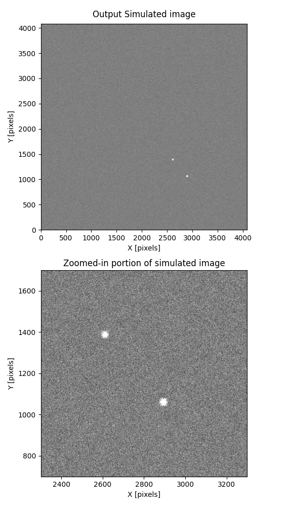
This output image was simulated with STIPS using this tutorial.
For additional questions not answered in this article, please contact the Roman Help Desk.
References
- Roman Research Nexus: https://roman.science.stsci.edu/hub/
- STIPS on readthedocs: https://stips.readthedocs.io/en/latest/
- STIPS on Github: https://github.com/spacetelescope/STScI-STIPS/tree/main
- STIPS Development Team et al 2024, "STIPS: The Nancy Grace Roman Space Telescope Imaging Product Simulator", PASP 136 124502