Visit Timing & Overhead Estimation

Proposers for the Roman Space Telescope can use the Astronomer's Proposal Tool (APT) to estimate the total time required to execute their science programs, including both science exposures and operational overheads. This article describes the Roman visit timing model and outlines the primary components that contribute to the time estimates reported by APT.
Overview
Both the Roman Astronomer's Proposal Tool (APT) and the Roman Planning and Scheduling Subsystem (PSS) use the Visit Timing Model to estimate the duration of an observation as executed onboard the observatory. APT provides users with several time estimates, each of which includes different categories of overheads, as described below. The values presented here are provided by the Roman Project and are based on simulations and current best estimates. These numbers will be updated after launch to reflect the observatory’s actual performance.
Improving Observing Efficiency
The Roman Science Operations Center (SOC) Planning & Schedule Subsystem is already optimized for operational efficiency, and users have limited ability to modify the sequence of observing activities or substantially reduce total overheads. Nevertheless, certain programmatic choices can help minimize overheads, even if the resulting gains are modest. General guidance is provided below, with links to more detailed discussions elsewhere in this article.
- The largest contributor to Roman observing overheads is the number of major slews in a program, along with the activities associated with each visit, including initial slews, guide star acquisitions, mechanism motions, frame resets, small angle maneuvers, and visit clean-up. Programs that minimize the number of major slews and the total number of visits will typically achieve a higher observing efficiency (science time divided by total time) than programs with many slews and visits.
- To the extent possible, users should group targets that can be scheduled together within the same observing segment. This grouping offers the most significant overhead reduction that APT can evaluate, and proposing observations that can be executed together generally leads to lower overall overheads
- To the extent possible, sequencing filters to minimize rotation of the element wheel assembly can further reduce overheads.
APT Time Estimates
APT provides several time estimates that include both science time and overheads, which are calculated at the visit level. In the context of Roman WFI observations, a segment consists of multiple visits and represents the smallest scheduling unit. A visit is a sequence of exposures executed without interruption, including small dithers and any required guide star acquisitions, corresponding to a single pass through a segment. For example, one visit typically corresponds to a single tile in a mosaic pattern.
In addition, overheads are categorized as either deterministic or statistical.
- Deterministic overheads are known in advance and are directly tied to the sequence of activities within a segment. Examples include guide star acquisition, mechanism motions, and small-angle maneuvers such as dithers or mosaics.
- Statistical overheads, in contrast, depend on the full scheduling context of Roman observations and cannot be precisely determined by APT alone. For example, a segment from one proposal may be interleaved with observations from other programs, making the actual slew preceding each segment unknown until final scheduling by PSS. To account for this uncertainty, statistical overheads include an assumed initial slew time for each segment.
APT reports time in three ways:
- Science Time includes the exposure specifications, excluding the reference reads.
- Execution Time includes the science time plus overheads with deterministic time estimates.
- Charged Time includes the execution time plus overheads that require statistical time estimates.
The Table of APT Time Estimates summarizes these time categories and indicates where they can be found within APT. The sections below provide a high-level overview of the Roman Visit Timing Model, which includes the Visit Science Duration (VSD) and the Initial Visit Overhead Duration (IVOD). We begin with an overview of the model itself, since both the VSD and IVOD incorporate slew and settle times.
Note
The specific numbers presented here are based off of APT 2025.6.2 (November 2025) and are subject to change.
Table of APT Time Estimates
| APT Time Estimates | Includes | Where to find in APT |
|---|---|---|
Science Time | Total science exposure time, excluding the reference reads. | Science Time for an individual pass is available under the Pass Plan. Total Science Time is available under Survey Plan and Program Information. |
| Execution time | Science Time plus:
| Individual pass Execution Time is available under the Pass Plan. Total Execution Time is available under Survey Plan. |
| Charged Time | Execution Time plus:
| Total Charged Time is available under Survey Plan and Program Information. |
Overview of the Roman Visit Timing Model
Slew & Settle Times
Slews to new targets, as well as inter-visit dithers and mosaic slews, are calculated using the slew and settle model shown in the Figure of Roman Timing Model for Slew and Settle. The total slew time depends primarily on the angular distance of the slews and is approximately linear for slews larger than ~1–2°. The Roman observatory’s settle time is short and nearly constant, varying only slightly between 8.5 and 9.0 seconds depending on slew size. As illustrative example, consider the following cases:
A 90° slew takes about 1,856 seconds, including settle time.
A 180° slew completes in just over one hour.
A 0° slew incurs a fixed overhead of 14.58 seconds.
A detailed Slew and Settle table that contributes to the Roman Timing Model implemented in APT is available on the Roman Technical Information Repository at /data/Observatory/SlewSettle/.
Figure of Roman Timing Model for Slew and Settle
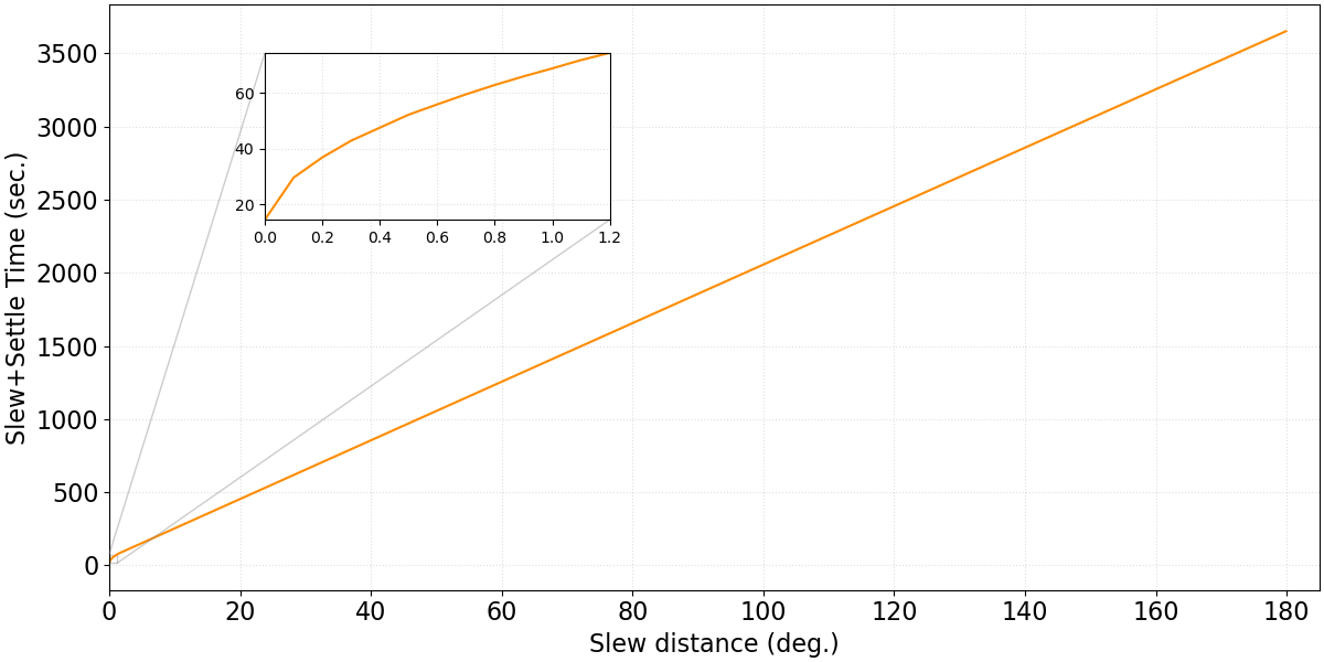
Roman slew and settle timing model, showing the total time to slew (and settle) as a function of the slew size. Except for small (i.e. <2 degrees) slews, the relationship is very close to linear. These values are based on modeling and are subject to change.
Table of Components in the Slew and Settle Calculation by APT
| Overhead | Includes | Total Duration (based on APT 2025.6.2 values and subject to change) |
|---|---|---|
Initial slew to target | Statistical average slew distance
| 444.33 seconds |
Slew time | Slew to target | see Figure below |
Settle time | Settling time once at target | About 9 seconds 2 seconds for slews < 0.00005° |
Dither overheads | Applies to both gap-filling and sub-pixels dithers | 0.2 second |
The elements contributing to the total slew and settle times computed in APT are summarized in the Table of Components in the Slew and Settle Calculation by APT. Because the initial slew to the first target in a segment cannot be known prior to actual scheduling (i.e. APT does not know what program will be observed immediately beforehand), a fixed statistical estimate is applied. The current statistical average slew distance is set to 20° (corresponding to ~453 seconds, including settle time), and is charged to the first visit of each segment. The statistical value will be updated in flight based on monitoring and calibration of the observatory’s attitude control system.
All subsequent slews, including slews to different targets within the same segment, as well as dithers and mosaic offsets, are calculated using the slew-and-settle model described below. An exception is made for very small slews: slews smaller than 0.00005° (less than 0.18 arcseconds) are assigned a fixed settle time of 2 seconds.
Note
Currently, time estimates for telescope rolls use the same model as translation slews. For example, a 5° roll is charged the time of a 5° slew. This approach slightly underestimates the time estimate and will be updated when possible.
Visit Science Duration (VSD)
The Visit Science Duration (VSD) is the total time from the start of the first science integration through to the end of the segment. This duration is deterministic and represents the sum of all the integration times, sub-pixel dithers, gap filling dithers, and end-of-visit activities. As summarized in the Table of Visit Science Duration Components, the VSD also includes additional overheads associated with constraint checks and loading the appropriate science MA table. If the integration is the final one in the visit, the VSD additionally includes the time required to configure the high-gain antenna (HGA) into tracking mode. When the Relative Calibration System lamp is used during an integration, an additional lamp turn-on warm-up time is also included.
Note
The VSD does not include the initial slew and slew settle time, or any additional time incurred by the WFI element wheel repositioning that might occur in parallel with the initial slew and settle time.
Table of Visit Science Duration Components
| Overhead | Includes | Total Duration |
|---|---|---|
Integration Start Overheads
|
|
|
| RCS warmup can take up to 60 seconds. | |
| Integration Time | Total integration time, including the reference read. | Based on MA Table used. |
| Dithers and Overheads | See Slew and Settle Times | Based on slew angle. |
| Integration end Overheads | High-gain antenna reconfiguration (for last integration of visit). | 2.0 seconds |
Initial Visit Overhead Duration (IVOD)
In addition to the VSD, the Initial Visit Overhead Duration (IVOD) accounts for the portion of the segment that occurs before science integrations begin. This includes the slew to the target, slew settle time, movement of the WFI filter wheel, and guide star acquisition. All of these steps all occur prior to the VSD part of the visit described above. Movement of the WFI element wheel movement is performed in parallel with the slew and settle sequence. As a result, only the longer of the two durations (slew/settle vs. filter wheel motion) is included in the IVOD:
IVOD = MAX\bigg( (slew\_ovrhd+slewtime+settle\_time), (filter\_move\_time+GSACQ\_time)\bigg)
Note that the filter wheel element is repositioned only at the start of a visit, and guide star acquisition can begin only after slew settling has started and the filter wheel movement is complete. The Figure of Breakdown of the Initial Visit Overhead Duration (IVOD) illustrates how these parallel overheads are incorporated into the IVOD.
Figure of Breakdown of the Initial Visit Overhead Duration (IVOD)
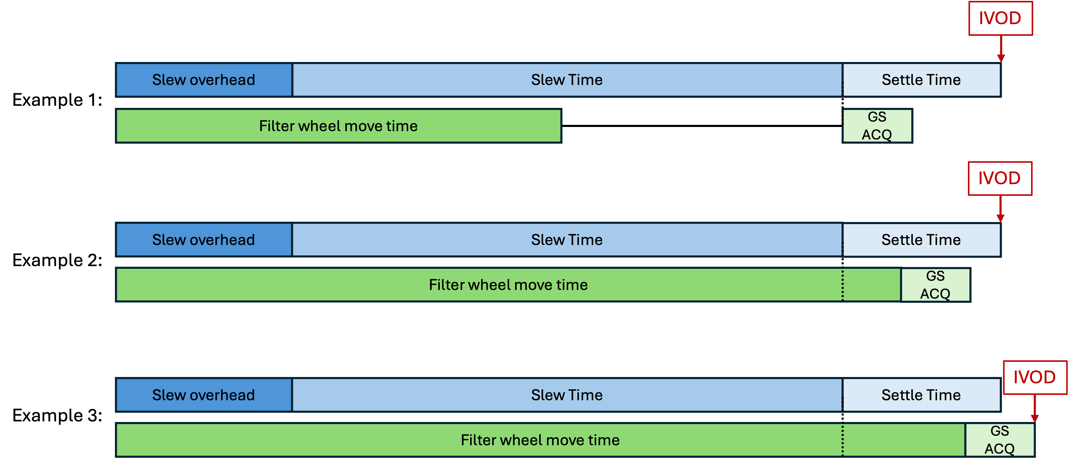
Breakdown of the initial visit overhead duration. Since some elements of the IVOD occur in parallel, the IVOD is the larger of (1) the slew and settle times and (2) the filter wheel move and guide star acquisition times.
Top and Middle: slew times are the larger contributors.
Bottom: filter wheel move and guide star acquisition times are the larger contribution. This cartoon representation of the IVOD is not to scale.
Filter Wheel Rotation
Filter wheel rotation times range from 0 to ~61 seconds and occur in parallel with the slew to the visit target. If the slew duration exceeds 61 seconds, the filter wheel rotation is fully contained within the slew time and introduces no additional overhead (see also the Figure of Breakdown of the Initial Visit Overhead Duration (IVOD)).
Since the Roman filter wheel assembly has a limited operational lifetime, users are encouraged, when possible, to sequence filters within a segment so as to minimize the total number of filter wheel rotations.
Figure of Approximate Roman Filter Wheel Element Move Times
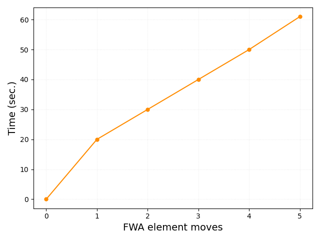
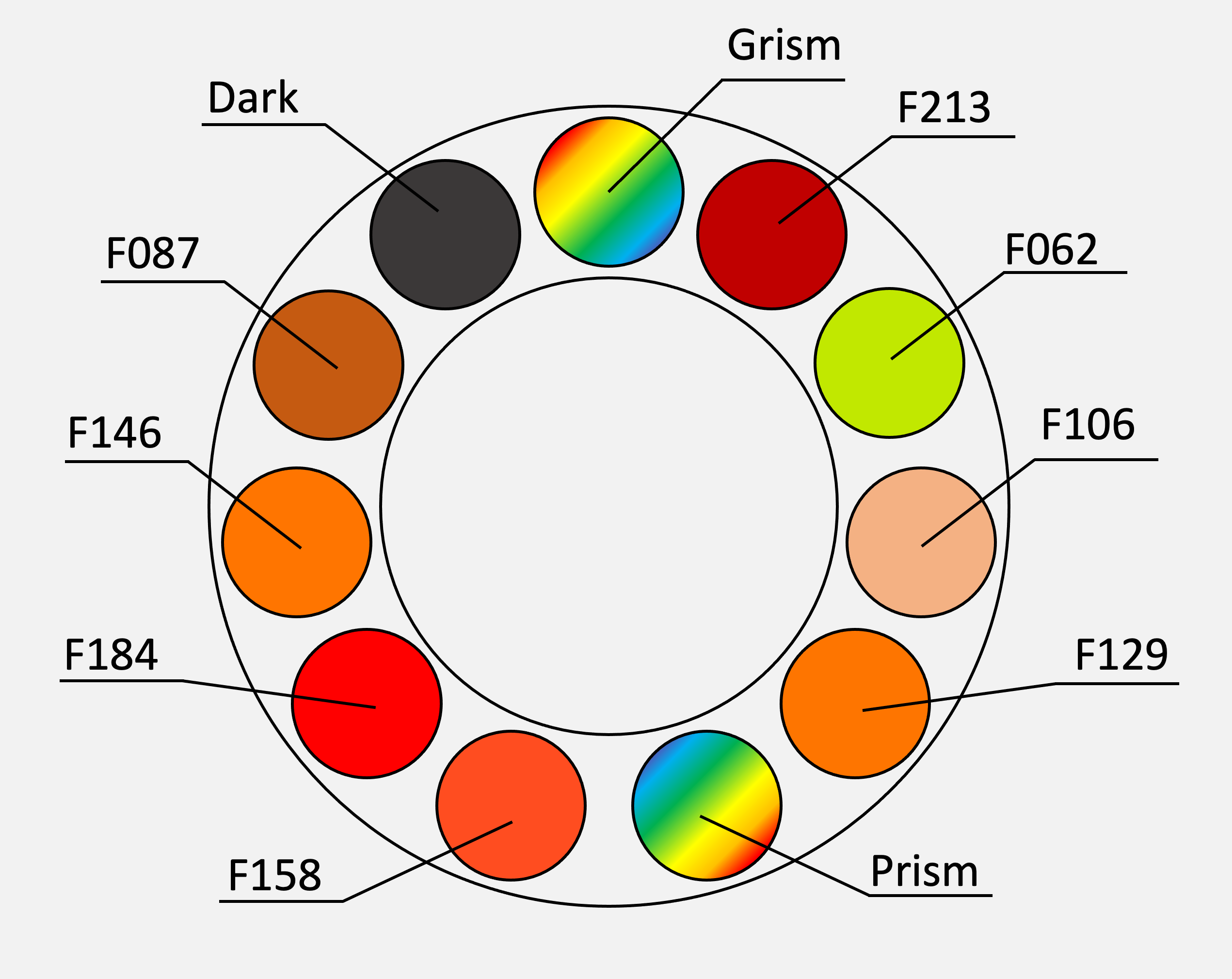
Top: Approximate times for moving the filter wheel assembly from one filter to another. The longest time to reach any EWA element is approximately 61 seconds (five element moves).
Bottom: Graphic of the locations of filters in the EWA with the optical elements labeled. Changing from the PRISM to GRISM is a five element move and would take 61 seconds.
Guide Star Acquisition
Guide star acquisition for Roman takes approximately 1 second. Any slew or dither larger than one WFI pixel (~0.11″) requires a guide star re-acquisition. The acquisition process may begin during slew settling, provided that movement of the filter wheel assembly has been completed.
Example Calculation of APT Time Estimates
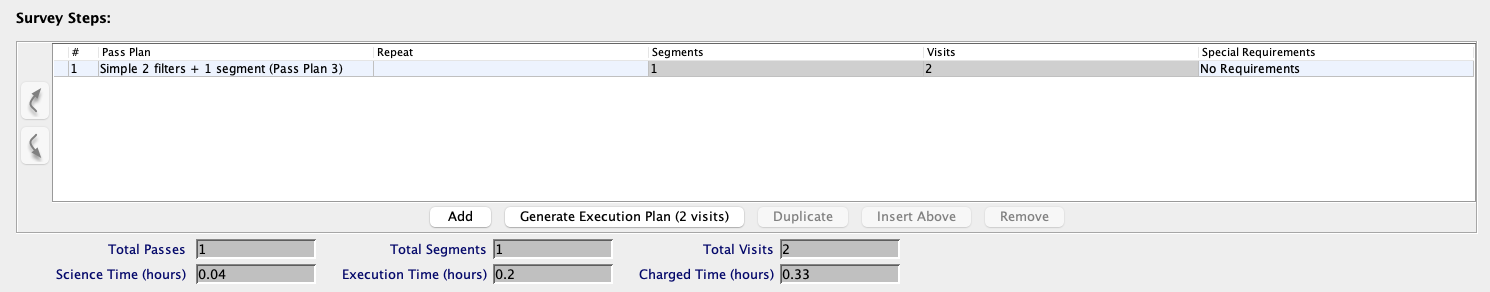
Below is an example illustrating how APT calculates the different time estimates for a simple program consisting of a single segment with two targets observed using different filters. The Figure of Simple Example of an APT Pass with Two Targets and Filters shows a screenshot of this APT program, along with the reported Science and Execution Times for the pass displayed.
Figure of Simple Example of an APT Pass with Two Targets and Filters
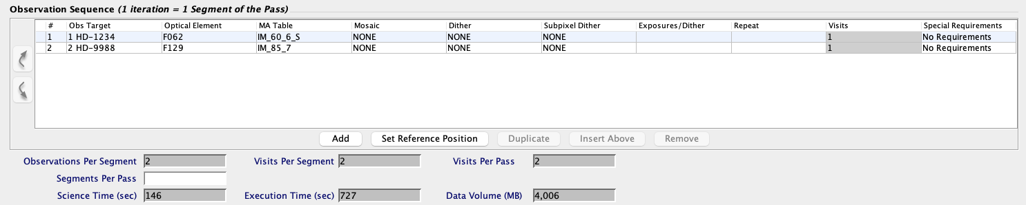
Simple example of an APT pass with two targets and filters, showing the Science and Execution times (top).
The Charged Time can be found under the Survey Plan and/or Program Information (bottom).
Science Time
The Science Time is calculated by summing the accumulated exposure times from all visits within a program. In this example, the Science Time is (60.09 + 85.39) = 145.48 sec. ≈ 146 sec. The total accumulated exposure time can be obtained from the Resultant drop-down menu in APT.
Execution Time
The Execution Time is defined as the sum of the Visit Science Duration (VSD) and the Initial Visit Overhead Duration (IVOD).
In this example, the VSD is calculated as the sum of instrument overheads, science integrations, high-gain antenna reconfiguration, and dithers. Since no dithers are included in this example program, the VSD is:
- Visit 1: (
3.5 + 63.25 + 2.0) = 68.75 seconds - Visit 2: (
3.5 + 88.55 + 2.0) = 94.05 seconds - The total VSD is therefore is
162.8seconds.
Note that the VSD includes the reference read (not shown in the APT’s MA Table menu), instrument overheads, and antenna reconfiguration.
The IVOD is defined as the longer of the slew-to-target duration and the filter wheel rotation time, with the guide star acquisition time added.
- The slew distance between the two targets can be obtained by exporting the APT Times report (see Additional Notes). In this example, the slew distance is
25.49°, corresponding to a slew time of554.52seconds. Adding9.0seconds of settle time and0.2second of overheads yields a total of563.72 seconds. - The filter wheel rotation between F062 and F129 takes approximately
29 seconds, and guide star acquisition requires1 second, for a total of30 seconds. - Since the slew and settle time is longer, the
IVOD = 563.72seconds. The total APT Execution time is therefore(VSD + IVOD) = (162.8 + 563.72) = 726.52 seconds ≈ 727 seconds.
Charged Time
Charged time adds the statistical initial slew estimate to the Execution Time.
In this example, the program contains a single segment with a statistical initial slew of 20°, corresponding to 444.33 seconds plus 9.0 seconds of settle time, for a total of 453.33 seconds.
As a result, the total Charged time is (726.52 + 453.33) = 1179.85 sec. = 0.328 hours ≈ 0.33 hours.
Additional Notes
For users seeking more detailed information about their program’s duration, APT allows the export of a “Times Report [.times]” via the File menu. In particular, the APT Times report provides the VSD and IVOD, along with a detailed breakdown of inter-segment and inter-visit overhead times.
Additionally, the Data Volume reported by APT is the sum of the science data volumes for each integration within a visit. The data volume for an individual integration is taken from the MA Table and depends on the number of resultants used in that integration. Note that the MA Table reports data volume in gigabits, whereas APT reports data volume in megabytes.
For additional questions not answered in this article, please contact the Roman Help Desk.
References
- Roman Technical Information Repository: https://github.com/RomanSpaceTelescope/roman-technical-information