Skymap Tessellation

Given the large data volume produced by Roman's surveys, the Roman Science Operations Center (SOC) has adopted a tessellation scheme to partition the celestial sphere. The Level 3 mosaic files in the Roman archive will be stored according to this tessellation.
Motivation
The Roman Space Telescope (Roman) will perform large, community-defined surveys with the Wide-Field Instrument (WFI) as well as general astrophysics surveys that can observe any part of the sky. During its mission, Roman will observe large areas of the celestial sphere. Therefore, it is useful to develop an optimal sky tessellation scheme to facilitate the generation of high-value scientific data products that are also easy to archive and retrieve.
The typical approach used in past optical and infrared surveys is to archive mosaics of sky regions created with a tangential projection. These regions are usually large enough to contain extended galaxies or other objects, have minimal overlaps, and can be stored in smaller components. These smaller components can be then retrieved and seamlessly combined into larger mosaics without requiring additional resampling.
A few surveys such as PanSTARRS and LSST use or plan to use the RINGS.V3 method, which is described in the Documentation for PS1 Sky Tessellation Patterns. Unfortunately, this method has some performance issues around the polar regions, where the tiling can leave gaps. Alternatively, the Euclid Space Telescope Collaboration opted for tessellations based on HEALPix (Euclid Collaboration, 2022), as did several other sky mapping missions that use HEALPix, including Planck and WMAP, which produced maps of the cosmic microwave background. The HEALPix projection is an elegant way to tessellate the celestial sphere with equal-area isolatitude tiles (Gorski et al. 2005). It divides the sky into rhomboid-shaped regions on a sphere, which are then subdivided into square sub-regions to create rectangular, north-oriented tiles. However, since these sub-regions follow diagonal boundaries, they only partially cover the projected region leading to inefficient data storage.
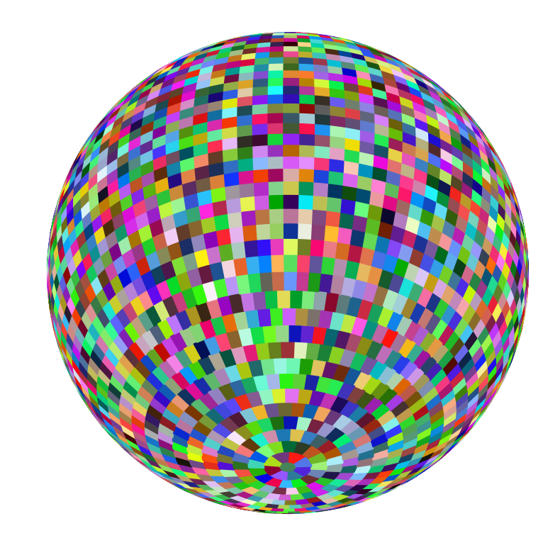
For Roman, we chose a tessellation method that combines the advantage of having rectangular tiles organized in rings with the elegance of the HEALPix tessellation (see the Figure of the Celestial Sphere). This was implemented by using the ”double pixelization” extension of HEALPix proposed by Calabretta & Roukema (2007).
Figure of the Celestial Sphere
Roman Tessellation Method
To fully appreciate the tessellation method chosen for Roman, it is helpful to first understand some foundational concepts behind HEALPix (Gorski et al., 2005) and the double-pixelization scheme proposed by Calabretta & Roukema (2007). These are summarized in the expandable section below.
HEALPix and Double Pixelization
An elegant way to achieve an equal-area, isolatitude tessellation of the sphere is to use the HEALPix projection (Gorski et al. 2005). A sphere can be partitioned with a regular rhomboidal grid consisting of N_{\theta} rings containing the centers of the rhombi subdivided in N_{\phi} equatorial cuts. There will be a N_{\theta}N_{\phi} number of tiles with area equal to \frac{4\pi}{N_{\theta}N_{\phi}}. Each side of a rhombus can then be subdivided in N_{side} parts to generate a hierarchical tessellation.
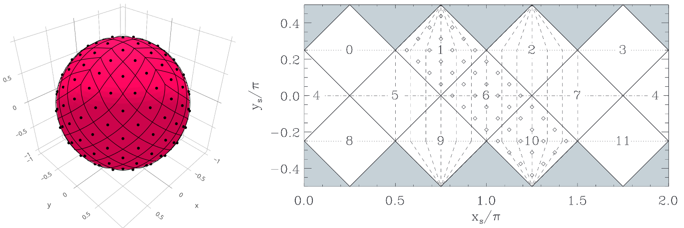
The optimal choice in cosmic microwave background surveys using HEALPix is to adopt N_{\phi}=4 and N_{\theta}=3 which subdivides the sphere in 12 diamond-shaped spherical polygons and leads to a pixelization with minimal distortion. Each rhombus can then be subdivided in N^{2}_{side} identical rhombi by dividing each side into N_{side} parts to reach the desired degree of resolution (see the HEALPix Tessellation Figure).
HEALPix Tessellation Figure
The area of each tile is therefore:
| \frac{4\pi}{N_{\theta}N_{\phi}N^{2}_{side}} = \frac{\pi}{3N^{2}_{side}} |
This means that to have tiles with a given angular size \alpha using a tessellation with N_{\phi}=4 and N_{\theta}=3, each rhombus must be subdivided N_{side}=⌈(\pi/3/\alpha)^{1/2}⌉ times, where the half brackets indicate the ceiling function, i.e. the least integer greater than or equal to the value in the brackets.
The projection is equivalent to a cylindrical equal-area projection in the equatorial region. In the polar region, however, the projection changes. To determine the transition latitude where this change occurs, note that the area of the polar cup at this latitude corresponds to one sixth of the total surface area of the sphere.
Assuming that the latitude angle \theta lies in the interval [-\frac{\pi}{2}, \frac{\pi}{2}], let \theta_x denote the transition latitude angle (i.e. where the projection changes). The area of the polar cup is then given by 2\pi(1-\sin\theta_x)=\frac{4\pi}{6}. Solving for \theta_x, we get:
| \theta_x = \sin^{-1} (2/3) \approx 41^o.81 |
As shown in the HEALPix Tessellation Figure, the sphere can be mapped onto the (x, y) plane using 12 square diamonds by setting N_{\phi}=4 and N_{\theta}=3. For a more compact representation, one of the equatorial diamonds is split into two parts. Points on the sphere with spherical coordinates (\phi, \theta) can be mapped to points to planar coordinates (x, y) using the following pseudo-cylindrical transformation.
| \mbox{A simple cylindrical transformation is used in the equatorial region, } |\sin \theta| \leq \frac{2}{3}: \\ \hspace{4em} x = \frac{\phi}{\pi} \\ \hspace{4em} y = \frac{3}{8} \sin \theta \\ |
| \mbox{While, in the polar regions, } |\sin \theta| > \frac{2}{3}: \\ \hspace{4em} x = \frac{\phi}{\pi} - (|2-\sqrt{3(1-\sin\theta)}|-1)\left(\left(\frac{\phi}{\pi} \mod \frac{1}{2}\right) -\frac{1}{4}\right)\\ \hspace{4em} y = \frac{2 -\sqrt{3(1-\sin\theta)}}{4} |
Conversely, planar coordinates can be converted to spherical coordinates with the following transformations.
| \mbox{In the equatorial region, } |y| \leq \frac{1}{4}: \\ \hspace{4em} \phi = \pi x \\ \hspace{4em} \sin \theta = \frac{8}{3} y \\ |
| \mbox{In the polar regions, } \frac{1}{4} < |y| < \frac{1}{2}: \\ \hspace{4em} \phi = \pi x - \pi \frac{|y|-1/4}{|y| - 1/2} \left(\left(x \mod\frac{1}{2}\right) - \frac{1}{4}\right) \\ \hspace{4em} \sin \theta = \left(1 - \frac{1}{3} ( 2 - 4|y|)^2\right) \frac{|y|}{y} \\ |
| \mbox{with x restricted to:}\\ \hspace{4em} \left|\left(x \mod\frac{1}{2}\right) - \frac{1}{4}\right| < \frac{1}{2} - |y| |
The primary drawback of this tessellation for imaging data is the unusual orientation of the tiles (diamonds rotated at 45 degrees).
To address this, Calabretta & Roukema (2007) proposed a method called ”double pixelization”, which produces tiles aligned with the sphere’s parallels and meridians. This is achieved by inserting an additional tile between each pair of tiles at the same latitude, along with two extra tiles at the poles. As a result, the total number of tiles increases from 12N^{2}_{side} to 24N^{2}_{side}+2. Each tile covers an area of \frac{\pi}{6N^{2}_{side}}, corresponding to half that of the standard HEALPix tile, except for the 8 corner tiles (two of which are marked with red arrows in the HEALPix Double Pixelization Figure), which each cover 75% of a standard tile. The remaining area is accounted for by the two polar tiles (see the HEALPix Double Pixelization Figure).
Despite this restructuring, it is possible to use the original HEALPix indexing scheme by doubling the HEALPix indices and incrementing them by one, so that the indices range run from 0 to 24N^{2}_{side}+1, with the first and last corresponding to the poles.
HEALPix Double Pixelization Figure
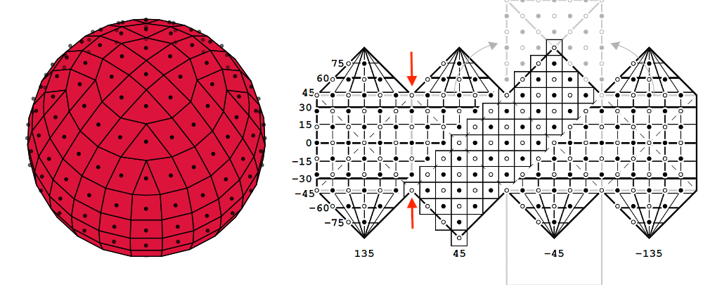
Double pixelization mapping with N_{side}=3. The sketch illustrates how the regions defined by the double pixelization are projected onto the plane as squares oriented along the sphere's parallels and meridians. On the sphere, the tiles are rectangular near the equator and progressively more slanted at higher latitudes.
Roman Tessellation
The HEALPix double pixelization method is designed to work with the HEALPix projection, which maps the sky in such a way that the diamond-shaped regions on the sphere become perfect squares onto a plane. However, the Roman Space Telescope uses a different approach, a tangential (or gnomonic) projection, to generate its mosaic products. Unlike the HEALPix projection, this method flattens the sky from a local viewpoint, which causes distortions that grow with distance from the projection center. As a result, the sides of tiles defined with the HEALPix double pixelization no longer align cleanly with lines of constant longitude (meridians), especially near the poles, where the distortion is most pronounced.
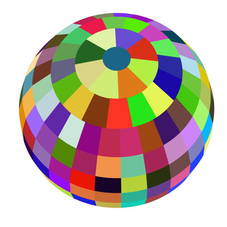
To define the Roman tessellation, tile centers and declination boundaries are derived using the HEALPix "double pixelization" scheme. The right ascension boundaries are then set as the midpoints between two consecutive centers at the same latitude. This method produces a straightforward tiling of the sphere, with most tiles being approximately rectangular and similar in size and area (see the Figure of Roman Tessellation). Some distortions from the ideal rectangular shape become noticeable near the poles, where the projected tile only partially fills the rectangular mosaic frame. Despite this, the resulting tiles remain fully symmetrical.
Figure of Roman Tessellation
Nomenclature
Large tiles are convenient for studying extended sources; however, smaller files are more efficient for storage, allowing easier retrieval of archived products and simplifying the production of source catalogs. For this reason, each tile is subdivided into smaller square patches. In this section we define the terms used in tessellation and mosaic creation. A graphical illustration is provided in the Figure of Skycells.
A sky tile (sometimes abbreviated as "tile") is a region on the spherical surface of the sky defined by the tessellation. Each sky tile is delimited in declination and right ascension and its center is used as the reference center for the gnomonic projection (see projection region definition below). Each sky tile is indexed according to the HEALPix double pixelization scheme. In the Figure of Skycells, sky tile #1000 is illustrated with dark green on the sphere.
A projection region, shown in the middle panel of the Figure of Skycells, represents the tangent-plane projection of a sky tile, with the tangent point located at the tile's center. We use a gnomonic projection, a tangential projection with the origin at the center of the sphere, in equatorial coordinates. In the Figure of Skycells, the boundaries of the projection region are marked as a dashed green line. Because the boundaries of a tile are defined as sides with constant latitude (top and bottom) and constant longitude (left and right), the lateral sides of the projection regions appear linear under the gnomonic projection, while the top and bottom sides are curved. For projection regions near to the equator (as in the figure), the latitude boundaries appear almost as straight lines. As one moves towards the poles, the bottom and top sides become increasingly curved, and the lateral sides increasingly tilted (see also Figure of Projection Region Shapes).
A sky cell is the square mosaic (Level 3) data product stored in the Roman Archive, and is a component of the projection region. Each projection region is subdivided into sky cells, each measuring 4.6 arcminutes per side. This size ensures that data product files remain of a reasonable disk size even when pixels are oversampled by a factor of 2 relative to the native pixel scale.
The core region of a sky cell is the set of pixels unique to the sky cell (which comes from the direct partition of the projection region).
The overlap region, defined with a width of 5 arcseconds, consists of the pixels that overlap with a adjacent, neighboring sky cell. This overlap region is useful for detecting slightly extended sources located near the border of a cell.
Figure of Skycells
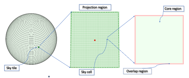
The 1,000th sky tile on the sphere shown as a projection region in a tangent plane and its component sky cells. A sky cell is shown in detail demonstrating the core region as well as the overlap region with its neighboring sky cells. The dashed green line around the projection region shows the limits of the projection region.
Details of the Implementation for Roman
Once a tessellation scheme is selected, the optimal sizes of the projected pixel, tile, and region must be determined.
Pixel Size
The size of the pixel is dictated by the detector's native pixel scale, which for the WFI, is 0.11 arcseconds per pixel. By applying the drizzle algorithm to reconstruct the point spread function (PSF) from a stack of suitably dithered images, it is possible to use pixels smaller than the native size to fully exploit subpixel dithering. This can result in pixel sizes that are half the native pixel scale. Even in cases of shallow coverage, it is advantageous to reproject the original images onto a finer pixel grid, since the orientation of the detector pixels may differ from that of the projection, leading to potential resolution loss. Therefore, an oversampled pixel size of 0.055 arcseconds per pixel was adopted. However, in cases where a slight loss of resolution is acceptable, the even number of pixels per cell makes it straightforward to revert to the native pixel size while maintaining the same tile and cell dimensions.
Tile size
The size of the tile depends on considerations related to the size of the array (i.e., the size of a pointed observation), the size of extended objects, and the amount of the distortion introduced by the projection.
Distortion
We consider here a gnomonic projection, a typical choice in astronomy, that projects the sphere on a tangential plane with the center of the sphere as reference point for the projection. The point where the tangent plane touches the sphere is called the projection center. The gnomonic projection is neither conformal nor equal-area. Shape, area, and distance distortions increase with distance from the projection center. It is therefore important to limit the size of the tile to have negligible distortion.
Figure Exploring Tile Distortion
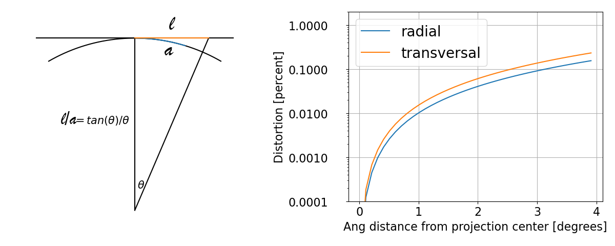
Distortion as a function of the distance from the center of projection for a tangential projection. The first panel explains the formula used for the computation. In the second, we can see that the distortion is negligible (less than 0.1%) up to 2°.
The projection stretches each radial arc of the sphere into a radial segment. As shown in Figure Exploring Tile Distortion, the ratio between a radial arc and its projection can be computed with simple trigonometry and it is equal to:
| \frac{l_r}{a_r} = \frac{\tan(\theta)}{\theta} |
where \theta is the angular distance from the projection center, a_r is the length of the arc on a circle passing through the projection center, and l_r the length of its projection. The length of a circle centered on the projection center is also stretched while projected. In this case, since the radius of the circle on the unit sphere is equal to \sin\theta and the radius of the circle on the tangential plane is equal to \tan\theta, the ratio between the length of the projected arc l_t and the one on the sphere is:
| \frac{l_t}{a_t} = \frac{1}{\cos(\theta)} |
As shown in Figure Exploring Tile Distortion, the distortion is less than 0.1% for distances from the center of projection smaller than 2 degrees, that is, for tiles with sides shorter than 4 degrees. Consequently, distances across the sphere in both radial and transverse directions increase with larger angular separations. For angles less than 2 degrees, the distortion in distance remains below 0.1%.
Figure Exploring Pixel Distortion
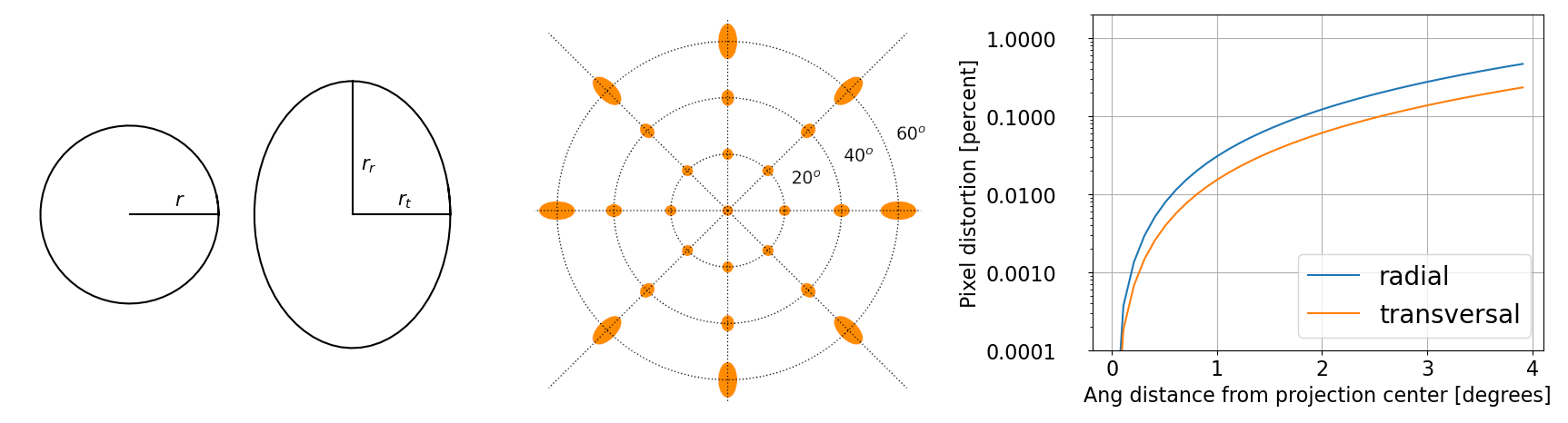
Circles on the sphere are distorted into ellipses when projected on the tangential plane. The middle panel shows the projection of an infinitesimal circle on the sphere in different locations (Tissot’s indicatrix) for a gnomonic projection. For angles smaller than 2 degrees, i.e., tiles with sides shorter than 4 degrees, the distortion in shape is less than 0.1%.
The projection also distorts shapes at different positions on the map. A useful way to visualize this shape distortion is by computing the projection of an infinitesimal circle on the sphere at various locations, a technique known as Tissot's indicatrix (see middle panel of Figure Exploring Pixel Distortion). Due to the symmetry of the gnomonic projection, the circle is mapped into an ellipse, with the major axis aligned along the direction pointing toward the projection center. The distortion can be quantified as the deviation from the original radius along the two axes of the resulting ellipses. The distortion is maximal in the radial direction and minimal in the transverse direction.
The transverse component will be stretched with the same ratio as the total circumference, so:
| \frac{r_t -r}{r} = \frac{1}{cos(\theta)} - 1 |
The stretch of the radial component can be computed by simply differentiating the length of radial ratio
| \frac{\partial{l_r}}{\partial{a_r}} = \frac{\partial{\tan{\theta}}}{\partial{\theta}} |
thus obtaining:
| \frac{r_r -r}{r} = \tan^2(\theta) |
As shown in the Figure Exploring Pixel Distortion, the maximal distortion of a pixel, the smallest element of a mosaic, is less than 0.1% for angular distances smaller than 2 degrees.
Extended Sources and Continuous Field of View
When studying large structures (e.g., galaxy groups, clusters, and superclusters), it is convenient to work with a single large image. Breaking up an extended source into multiple tiles poses a significant challenge, as it requires reprojecting adjacent fields to reconstruct its full image. The right panel of the Figure to Select Tile Size shows the probability of imaging a galaxy the size of the Andromeda galaxy (∼50 kpc) within a single tile, as a function of redshift. Assuming a tile size of 3.2 degrees by 3.2 degrees, galaxies smaller than 12 arcminutes fit within a single tile more than 90% of the time. Messier objects, which are typically smaller than 10 arcminutes, will fall within a single tile of 3.2 degrees by 3.2 degrees more than 90% of the time. Smaller tiles are more likely to break extended objects into multiple tiles.
Figure to Select Tile Size
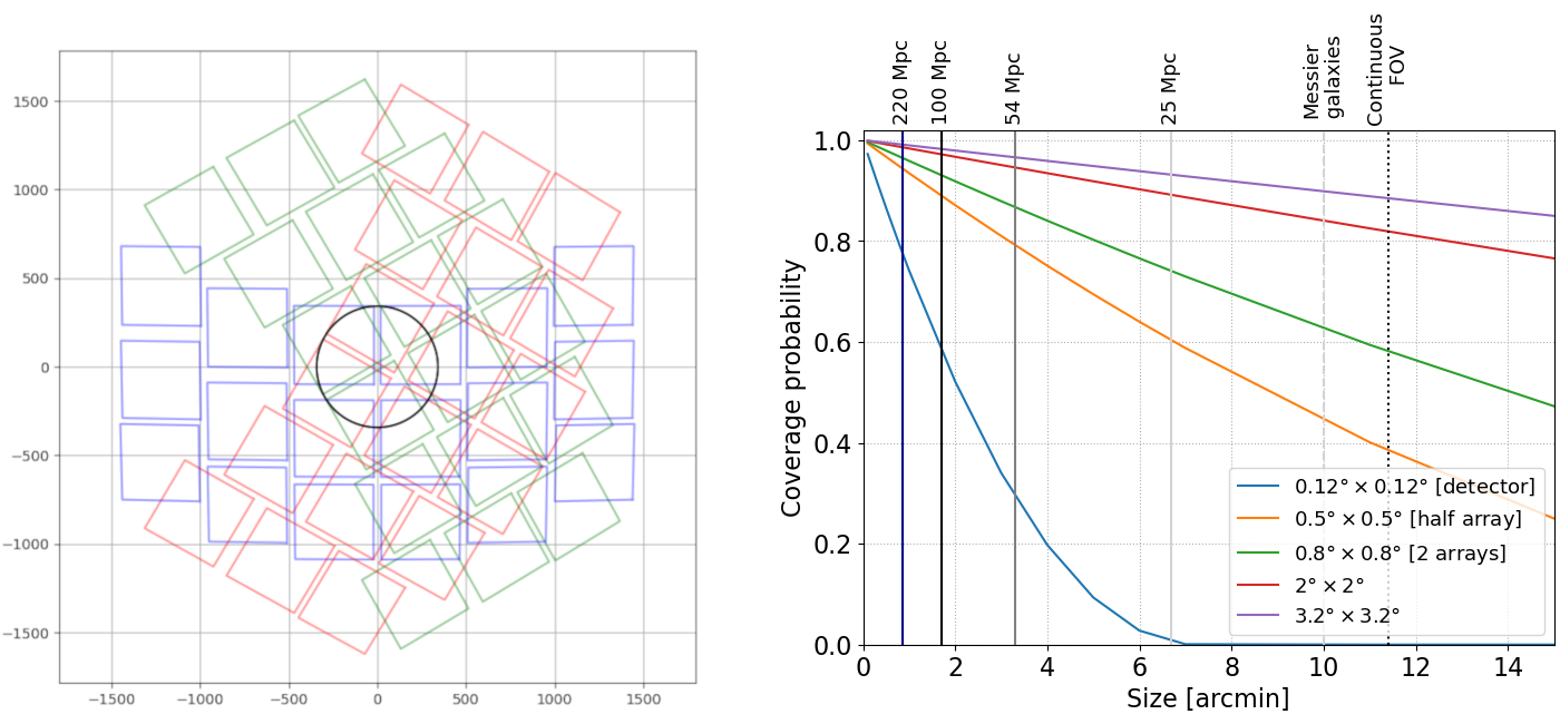
Left: Footprint of the WFI rotated at three angles to simulate three random observation times. The minimal dithering to cover the gaps between detectors is shown in one case (blue footprint). The continuous WFI field of view (FOV) is traced with a black circle. Right: Probability that Andromeda–size galaxies (~ 50 kpc diameter) at various distances, Messier-type galaxies, and the continuous FOV of the WFI lie entirely within a sky tile of a given size. Each color corresponds to a different tile size.
Another important factor in determining the tile size is the size of the continuous field of view, defined as the area of the sky with homogeneous coverage when the focal plane is pointed at a given position across multiple orientations (or epochs) and after applying gap-filling dithers. An example is shown in the left panel of the Figure to Select Tile Size, where the focal plane is observed at three random epochs (orientations). The continuous field of view corresponds to a circular area with a diameter of 11.4 arcminutes (depicted by the black circle in the Figure to Select Tile Size). Assuming a tile size of 3.2 degrees by 3.2 degrees, the probability that the continuous field of view falls entirely within a single tile is approximately 90%.
Based on these considerations, a tile size with a side of 3.2 degrees was deemed appropriate, as it is large enough to support scientific investigations while remaining small enough to minimize distortion effects on peripheral pixels.
Size of the Projection Regions
Once the sky tile is determined, the next step is to define the size of the projection regions. Although the areas of the sky tiles are very similar by design, their sizes vary from the equator to the poles (see Figure of Sky Tile Sizes). The projection regions have a maximum x-dimension of 297,409 pixels and a maximum y-dimension of 282,252 pixels. By adopting sky cells with sides of 4,800 pixels and using the oversampled pixel scale of 0.055 arcseconds per pixel, the projection region can be covered with a maximum of 62 cells in the longitudinal (x) direction and 59 in the latitudinal (y) direction. To facilitate source extraction, it is beneficial to include an overlapping region of approximately 10 arcseconds between adjacent sky cells. This requires adding a 5-arcsecond-wide overlapping region around each cell, corresponding to approximately 100 pixels at the oversampled pixel scale of 0.055 arcseconds per pixel. each sky cell will have a file size of 5,000 pixels by 5,000 pixels. In the cases where a minimal loss of resolution is not an issue, since the number of pixels for each cell is even, it is easy to revert to a native pixel size while maintaining the same size of tiles and cells.
Figure of Sky Tile Sizes
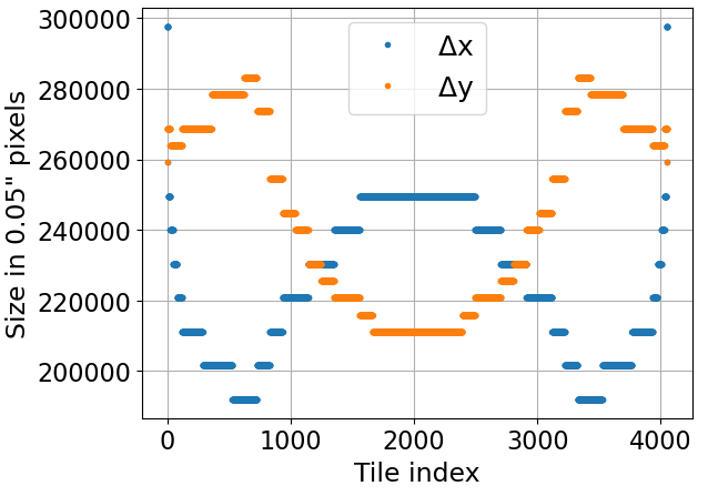
A plot of the x and y sizes of the smallest rectangular mosaic containing the tangential projection of the sky tile.
The Figure of Projection Region Shapes shows how the shape of the projection region changes with the latitude. The polar regions are circular, while areas near the poles are trapezoidal. As the distance from the poles increases, the projection regions become increasingly rectangular. Each projection region is subdivided into square sky cells that are archived.
Figure of Projection Region Shapes
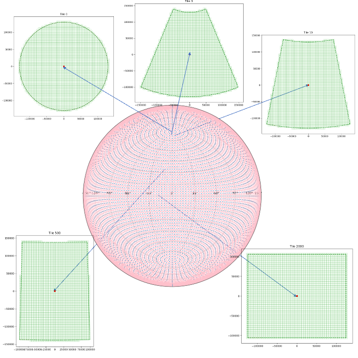
The tessellated sphere shown in Lambert projection with projection centers shown as blue dots. Sky tiles at different latitudes are shown tangentially projected as projection regions. The limit of a projection region is marked with a dashed green line. Each projection region is further divided into square sky cells, marked with solid green lines, which are archived as single files. The coordinates have the origin in the projection center (red dots in the projection regions).
For additional questions not answered in this article, please contact the Roman Help Desk.
References
- HEALPix Team Website, Sourceforge.io site maintained by the HEALPix Developers, Latest update 29 July 2022
- "Mapping on the HEALPix grid," Calabretta & Roukema 2007
- "HEALPix: A Framework for High-Resolution Discretization and Fast Analysis of Data Distributed on the Sphere," Gorski et al., 2005
- "Euclid preparation. I. The Euclid Wide Survey," Euclid Collaboration 2022
- "The Roman tessellation of the celestial sphere", Fadda et al., 2025, Technical Report Roman-STScI-000708