Synphot for Roman

Software Freeze: To ensure a stable user experience, updates to certain Roman tools will be suspended from June 28, 2026 through commissioning. Exceptions may be made for urgent fixes. Users will be notified of any releases made during this period.
Synphot Overview
synphot (STScI Development Team 2018) is a general software developed by the Space Telescope Science Institute that provides tools for the generation, manipulation, and simulated observation of a source based on its spectral properties. synphot is a Python package, and is an improvement upon previous, similarly named software that now incorporates features from astropy , such as astropy.units and astropy.modeling .
Note that JWST filters, if desired for any use cases, are only available through STPSF , although this may change in the future.
Code Repository and Documentation
The synphot code is publicly developed on GitHub, and the technical documentation on readthedocs includes additional information on the capabilities and use of synphot . Users are encouraged to open issues on the GitHub repository to give feedback or report problems.
Installation
synphot is installable via pip.
Basic installation of synphot on a Unix-like operating system using a Conda environment manager can be accomplished in a shell by typing the following:
$ conda create -n <environment_name> python
$ conda activate <environment_name>
$ pip install synphot
Note that the $ symbol indicates the prompt. The variable <environment_name> is at the discretion of the user. By indicating the argument "python" during the environment creation, the latest available version of Python will be installed in the environment along with other necessary tools such as pip.
stsynphot
Another Python package named stsynphot (STScI Development Team 2020) is used to load observatory-specific throughput curves, such as those from Roman and many other facilities. Available photometric systems are documented in Appendix B of the stsynphot readthedocs documentation. Alternatively, throughput information for the Roman WFI and James Webb Space Telescope instruments may also be retrieved from STPSF and loaded into synphot . For more information on how to install STPSF , see STPSF for Roman.
Similar to synphot , stsynphot is installable via pip. In the same environment that you installed synphot , type the following:
$ pip install stsynphot
The data files necessary for stsynphot include the Roman WFI throughput curves, spectral template and model libraries, and calibration reference spectra. More information on the supporting files, which are contained in several compressed TAR directories, can be found in Table 1 of the Spectral Atlas Files for Synphot Software documentation. In particular, the file labeled synphot1_throughput-master.tar from Table 1 contains the throughput curves for the Roman WFI, as well as other facilities such as Hubble, Sloan, and 2MASS among others.
You must have a copy of a Vega spectrum for several synphot functions to work. A version of a Vega spectrum is available in synphot6_calibration-spectra.tar from Table 1 of the Spectral Atlas Files for Synphot Software page.
Users must also set an environment variable called
PYSYN_CDBS
to point to the directory where these ancillary files are located. When uncompressing the TAR files, they should produce a subdirectory ending with /trds. To set the path to these files in a bash shell, type:
export PYSYN_CDBS = /path/to/my/trds
Then, replace the path with the appropriate path to the files on the system. This environment variable may be added to your startup files to ensure that it is set every time. Users who use conda as an environment manager may also save this as part of the environment.
Use Cases & Examples
Plot the Roman WFI Filter Throughputs and Information
There are two approaches to retrieving WFI throughput information, both of which should give the same results. Here we will show both methods of loading the WFI throughput information, and then show the remaining steps independent of that choice.
Before running the code cells below, we need to import several packages:
import os

from astropy import units as u
from astropy.time import Time
from matplotlib import pyplot as plt
import numpy as np

import synphot as syn
import stsynphot as stsyn
import stpsf
Retrieving WFI Throughputs from STPSF
To retrieve the optical element throughput information from
STPSF
, we set up the WFI object, and use the method _get_synphot_bandpass, which takes the optical element name as the only argument. For a list of optical elements, see WFI Optical Elements. In the example below, we load the throughput information from the F129 imaging filter. This new Python object behaves as a callable function that takes as input the wavelength or frequency of interest, and will return the throughput at that wavelength or frequency.
# Set up the Roman WFI object and retrieve the throughput of a filter
roman = stpsf.WFI()
wfi_f129 = roman._get_synphot_bandpass('F129')
print(wfi_f129(1.29 * u.micron))
Running this should yield approximately 0.6448.
Retrieving WFI Throughputs using stsynphot
Alternatively, we can also get information about the bandpasses using the following methods on the bandpass objects in stsynphot :
band = stsyn.band('roman, wfi, f129')
print('WFI F129:')
print(f'\tBandwidth: {band.photbw():.5f}')
print(f'\tPivot wavelength: {band.pivot():.5f}')
print(f'\tFWHM: {band.fwhm():.5f}')
print(f'\tThroughput at 1.29 um: {band(1.29 * u.micron):.4f}')
Running the above code block should yield something like the following:
WFI F129:
	Bandwidth: 942.49697 Angstrom
	Pivot wavelength: 12901.34508 Angstrom
	FWHM: 2219.41077 Angstrom
	Throughput at 1.29 um: 0.6448
Plotting and Computing Bandpass Information
Regardless of the method we chose to load the throughput data, we can then plot the throughput curves and compute some information about our bandpasses. The following code block will generate a plot of the WFI imaging filter throughputs (except F146, which has been omitted for clarity as it is much wider than the others):
# Set up the Roman WFI object and make a list of the optical element names
roman = stpsf.WFI()
roman_filter = ["F062", "F087", "F106", "F129", "F158", "F184", "F213"]

# Set up wavelengths from 0.4 to 2.5 microns in increments of 0.01 microns.
waves = np.arange(0.4, 2.5, 0.01) * u.micron

# Set up figure
fig, ax = plt.subplots()

# For each optical element, plot the throughput in a different color
# and shade the area below the curve.
colors = plt.cm.rainbow(np.linspace(0, 1, len(roman_filter)))

for i, f in enumerate(roman_filter):
    band = roman._get_synphot_bandpass(f)
    clean = np.where(band(waves) > 0)

    ax.plot(waves[clean], band(waves[clean]),
            color=colors[i])

    ax.fill_between(waves[clean].value,
                    band(waves[clean]).value,
                    alpha=0.5,
                    color=colors[i])

# Set plot axis labels, ranges, and add grid lines
ax.set_xlabel(r'Wavelength ($\mu$m)')
ax.set_ylabel('Throughput')

ax.set_ylim(0, 1.05)
ax.set_xlim(0.4, 2.5)

ax.grid(':', alpha=0.3)

plt.show()
Running the above code should generate a plot like the Figure of the WFI Filter Throughputs:
Figure of the WFI Filter Throughputs
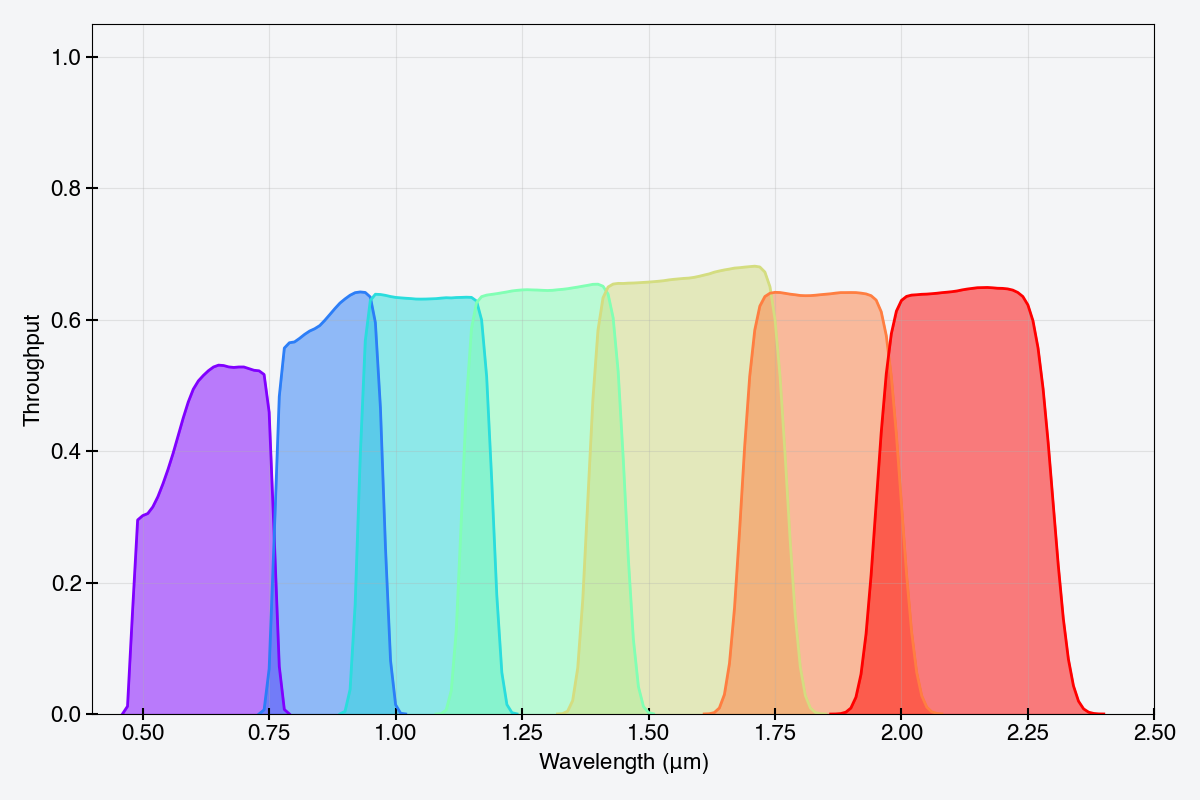
The throughputs of the WFI imaging filter elements have been plotted (omitting F146) as a function of wavelength in units of microns.
Synthetic Photometry of a Simulated Source
Here we show how to perform synthetic photometry of a simulated source. For this example, we will use a star of spectral type M5III, and we will add additional extinction to the source spectrum using the Milky Way extinction law.
# Load the WFI F158 element
wfi_f158 = stsyn.band('roman, wfi, f158')

# Retrieve the spectrum of the star
star_spec = syn.SourceSpectrum.from_file(os.path.join(os.environ['PYSYN_CDBS'], 'grid', 'pickles', 'dat_uvk', 'pickles_uk_100.fits'))

# Renormalize the spectrum to have a Johnson V-band magnitude of 22.5 ABmag
norm_spec = star_spec.normalize(22.5 * u.ABmag, band=stsyn.band('johnson, v'))

# Add extinction corresponding to E(B-V) = 2.3 using the Milky Way extinction law (Rv = 3.1)
extinction = syn.ReddeningLaw.from_extinction_model('mwavg').extinction_curve(2.3)
final_spec = norm_spec * extinction

# Compute the flux density arrays
wavelengths = np.arange(0.5, 2.5, 0.001) * u.micron
norm_fluxes = norm_spec(wavelengths, flux_unit=u.Jy)
final_fluxes = final_spec(wavelengths, flux_unit=u.Jy)

# Plot the spectra
fig, ax = plt.subplots()
ax.plot(wavelengths, norm_fluxes,
        color='blue',
        lw=2,
        label='Normalized Spectrum, V = 22.5 ABmag')

ax.plot(wavelengths, final_fluxes,
        color='red',
        lw=2,
        label=r'Reddened Spectrum, E(B $-$ V) = 2.3')

ax.legend()

ax.set_ylabel('Flux Density (Jy)')
ax.set_xlabel(r'Wavelength ($\mu$m)')

plt.show()
Running the above code block should produce a plot similar to the Figure Showing the Example Spectrum:
Figure Showing the Example Spectrum
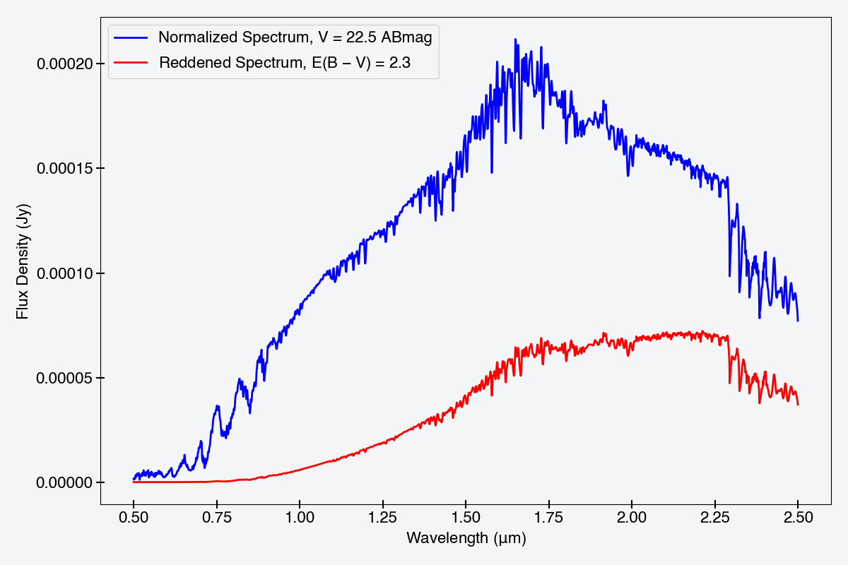
The blue line shows the spectrum normalized to a Johnson V-band AB magnitude of 22.5, while the red line shows the normalized spectrum after applying the Milky Way extinction law (RV = 3.1) to the normalized (blue) spectrum.
Now that we have our spectrum, we can "observe" it using the WFI:
# Observe the spectrum with the F158 bandpass
obs_spec = syn.Observation(final_spec, wfi_f158)

# Print out the magnitudes, flux density, and count rate (electrons per second) of the observed source
print('M5III star, WFI F158:')
print(f'\t{obs_spec.effstim(syn.units.VEGAMAG, vegaspec=syn.SourceSpectrum.from_file(syn.conf.vega_file))}')
print(f'\t{obs_spec.effstim(u.ABmag)}')
print(f'\t{obs_spec.effstim(u.Jy)}')
print(f'\t{obs_spec.countrate(area=np.pi * (2.4 * u.m)**2)}')
Running the above code block should yield something like:
M5III star, WFI F158:
	18.39474560651015 mag(VEGA)
	19.699190738813893 mag(AB)
	4.789869756452089e-05 Jy
	2188.783781214845 ct / s
For additional questions not answered in this article, please contact the Roman Help Desk.
References
- STScI Development Team 2018, Astrophysics Source Code Library. ascl:1811.001 https://ascl.net/1811.001
- STScI Development Team 2020, Astrophysics Source Code Library. ascl:2010.003 https://ascl.net/2010.003