The Wide Field Instrument (WFI) has a number of optical elements that are used for imaging and dispersive/spectroscopic scientific applications. These elements include the element wheel assembly with the filters: Grism, F213, F062, F106, F129, Prism, F158, F184, F146, F087, and Dark. Their properties are described in this article.

Element Wheel Assembly

The Wide Field Instrument (WFI) optical element wheel houses a set of eight imaging filters, two spectral dispersers, and a blank position, which are collectively referred to as optical elements (sometimes simply shortened to elements). The Figure of the Element Wheel Assembly with the Optical Elements Labelled presents the Element Wheel Assembly and shows the order of the optical elements.

The properties of the optical elements are described below in Table of Properties for Imaging Elements for imaging and the Table of Properties for Dispersive Elements for spectroscopy. Refer to the section on Bandpass Column Definitions for the equations that define each column in Table of Properties for Imaging Elements.

The blank position is not described in detail, however this is only rarely used for certain internal calibration modes, and is referred to as DARK in both the Astronomer's Proposal Tool (APT) and in the WFI data products. In APT, the DARK element is normally excluded from the list of selectable optical elements except for certain observing specifications (see the Calibration article in the Roman APT User Guide for examples of these modes).

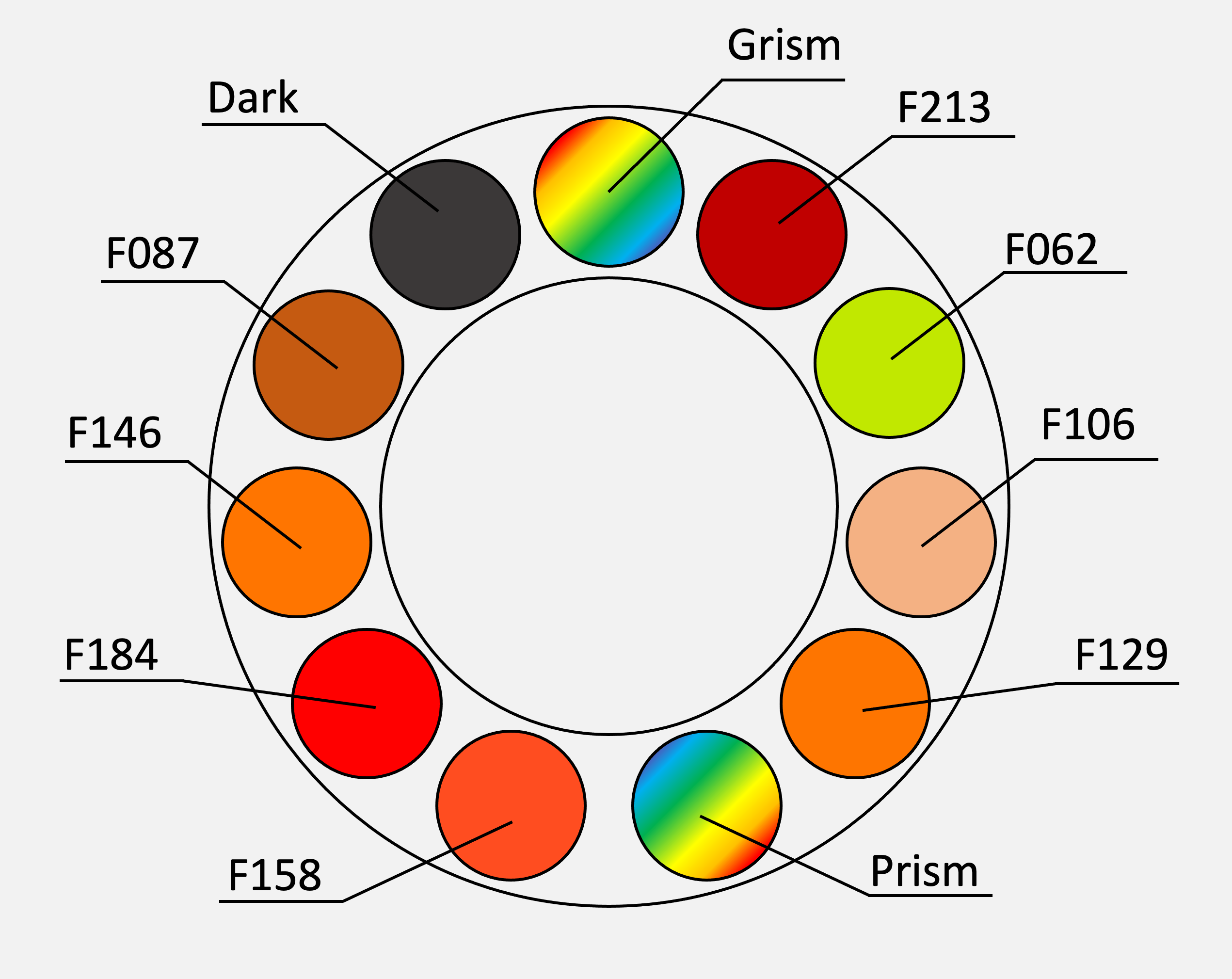
Schematic of the Element Wheel with each the optical elements labelled. From the top position and going clockwise the elements are: Grism, F213, F062, F106, F129, Prism, F158, F184, F146, F087, and Dark. The detailed properties of these elements are presented in this article.

Imaging Elements

The Table of Properties for Imaging Elements contains the detailed filter properties for each the imaging elements and the Figure of Properties for Imaging Elements displays the throughput curves (effective area) for each of the imaging elements.

The Roman Space Telescope Technical Information Repository v1.1 (Jan 30, 2025) contains additional information. For the spectroscopic mode, /data/WideFieldInstrument/Spectroscopy/Elements has the overall parameters, /data/WideFieldInstrument/Spectroscopy/Sensitivity has sensitivity estimates, /data/WideFieldInstrument/Spectroscopy/EffectiveAreas provides effective area tables for the position of each detector in the focal plane for each element.

Analogous filters from other systems are listed for informational purposes only. The WFI optical elements do not perfectly correspond to any of these other filters, and care should be taken to understand the differences between the WFI photometric system and other systems.

Table of Properties for Imaging Elements

Optical Element	Mean Wavelength (µm)	Pivot Wavelength (µm)	Bandpass Width (µm)	Bandpass FWHM (µm)	Bandpass RMS (µm)	Equivalent Width (µm)	Analogous Ground Filter
F062	0.6340	0.6291	0.0788	0.1856	0.0773	0.1243	R
F087	0.8719	0.8696	0.0633	0.1490	0.0632	0.1272	z
F106	1.0595	1.0567	0.0774	0.1823	0.0777	0.1632	Y
F129	1.2936	1.2901	0.0942	0.2219	0.0945	0.2022	J
F158	1.5791	1.5749	0.1152	0.2712	0.1154	0.2549	H
F184	1.8418	1.8394	0.0939	0.2210	0.0940	0.1966	H/K
F213	2.1255	2.1230	0.1038	0.2443	0.1039	0.2181	K_s
F146	1.4724	1.4378	0.3052	0.7188	0.3104	0.6854

Work is still on-going to align this content with the data provided in Roman Space Telescope Technical Information Repository v1.1 (Jan 30, 2025).

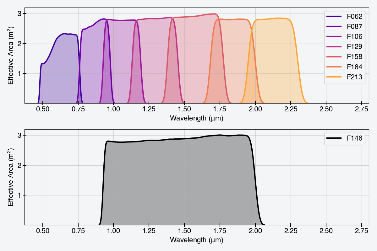
Effective area curves for the each of the imaging filters. The upper panel shows the seven normal-width filters and the lower panel shows the wide filter. The effective area curve for F146 is shown in a separate panel to aid in visibility. The effective area curves represent the total system throughput for a typical detector multiplied by the collecting area. The axis limits in all figures of optical elements are identical for reference.

Dispersive Elements

The Table of Properties for Dispersive Elements contains the optical properties of the prism and grism, while Figure of Properties for Dispersive Elements displays the effective area curves of the grism first order and of the prism. Throughput information for other orders is not available at this time, but may be provided in the future.

The Roman Space Telescope Technical Information Repository v1.1 (Jan 30, 2025) contains additional information. For the spectroscopic mode, /data/WideFieldInstrument/Spectroscopy/Elements has the overall parameters, /data/WideFieldInstrument/Spectroscopy/Sensitivity has sensitivity estimates, /data/WideFieldInstrument/Spectroscopy/EffectiveAreas provides effective area tables for the position of each detector in the focal plane for each element.

Table of Properties for Dispersive Elements

Optical Element	Minimum Wavelength (µm)	Maximum Wavelength (µm)	Center Wavelength (µm)	Width (µm)	R (per 2 pixels)
Grism	1.0	1.93	1.465	0.930	461
Prism	0.75	1.80	1.275	1.05	80 – 180

Release Tag

The information in this table corresponds to the Roman Space Telescope Technical Information Repository v1.1 (Jan 30, 2025).

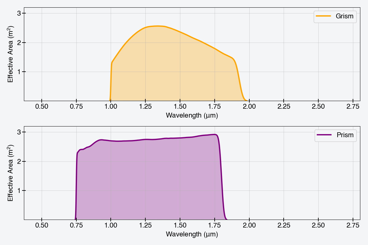
The figure contains two plots. Both plots are wavelength in microns on the X axis and the effective area in meters squared on the Y axis. The top plot shows the effective area curve for the grism in yellow, and the bottom plot shows the prism curve in purple. — Effective area curves of the grism first order and of the prism. The effective area curves represent the total system throughput for a typical detector multiplied by the collecting area. The axis limits in all figures of optical elements are identical for reference.

Bandpass Column Definitions

The columns in Table of Properties for Imaging Elements can be computed using synphot (STScI Development Team, 2018); more information about synphot can be found in the Synphot for Roman article. They are defined in the documentation as the following equations. In the equations below, $\begin{array}{l}P_\lambda\end{array}$ refers to the dimensionless bandpass throughput at a given wavelength $\begin{array}{l}\lambda\end{array}$ .

Mean wavelength (synphot.bandpass.avgwave()) is the average wavelength defined in Koornneef et al. (1986) on page 836:

$\begin{array}{l}\displaystyle \lambda_0 = \dfrac{\int P_\lambda \lambda\ \mathrm{d}\lambda}{\int P_\lambda\ \mathrm{d}\lambda}.\end{array}$

Pivot wavelength (synphot.bandpass.pivot()):

$\begin{array}{l}\displaystyle \lambda_{\mathrm{pivot}} = \left[\dfrac{\int P_\lambda \lambda\ \mathrm{d}\lambda}{\displaystyle\int\left(\dfrac{P_\lambda}{\lambda}\right)\ \mathrm{d}\lambda}\right]^{1/2}.\end{array}$

Bandpass width (synphot.bandpass.photbw()):

$\begin{array}{l}\displaystyle \mathrm{bw} = \bar{\lambda}\ \left[\dfrac{\displaystyle\int\left(\dfrac{P_\lambda}{\lambda}\right)\ln\left(\dfrac{\lambda}{\bar{\lambda}}\right)\ \mathrm{d}\lambda} {\displaystyle\int\left(\dfrac{P_\lambda}{\lambda}\right)\ \mathrm{d}\lambda}\right]^{1/2},\end{array}$

where $\begin{array}{l}\bar{\lambda}\end{array}$ is the mean log wavelength (synphot.bandpass.barlam()) from Schneider, Gunn, and Hoessel (1983), which is defined as:

$\begin{array}{l}\displaystyle \bar{\lambda} = \exp\ \left[\dfrac{\displaystyle\int\left(\dfrac{P_\lambda}{\lambda}\right)\ln(\lambda)^2\ \mathrm{d}\lambda} {\displaystyle\int\left(\dfrac{P_\lambda}{\lambda}\right)\ \mathrm{d}\lambda}\right].\end{array}$

Bandpass full-width half-max (FWHM; synphot.bandpass.fwhm()):

$\begin{array}{l}\displaystyle \mathrm{fwhm} = \mathrm{bw}\ \left[8\log(2)\right]^{1/2},\end{array}$

where bw is the bandpass width defined above.

Bandpass root mean square (RMS) width (synphot.bandpass.rmswidth()), which is defined in Koornneef et al. (1986) on page 836:

$\begin{array}{l}\displaystyle \lambda_{\mathrm{rms}} = \left[ \dfrac{\int P_\lambda\left(\lambda - \lambda_0\right)^2\ \mathrm{d}\lambda}{\int P_\lambda\ \mathrm{d}\lambda}\right]^{1/2},\end{array}$

where $\begin{array}{l}\lambda_0\end{array}$ is the bandpass average wavelength defined above.

Bandpass equivalent width (synphot.bandpass.equivwidth()):

$\begin{array}{l}\displaystyle \mathrm{eqw} = \int P_\lambda\ \mathrm{d}\lambda.\end{array}$

For additional questions not answered in this article, please contact the Roman Help Desk at STScI.

References

"Synthetic photometry and the calibration of the Hubble Space Telescope.", Koornneef, J. et al. 1986
"CCD photometry of Abell clusters. I. Magnitudes and redshifts for 84 brightest cluster galaxies.", Schneider, D. P., Gunn, J. E., and Hoessel, J. G. 1983
STScI Development Team 2018, Astrophysics Source Code Library. ascl:1811.001 https://ascl.net/1811.001

Latest Update	20 Dec 2024	Updated to align with the Roman Space Telescope Technical Information Repository.
Publication	05 Jan 2024	Initial publication of the article.

WFI Optical Elements